RNNによるクラス分類
RNNは中間層に再帰構造を持つニューラルネットで系列データの特徴を捉えることができるため、自然言語や音声、動画といった時系列を扱うことを得意としています。
RNNの構造は以下のようになっている。ただし、xは入力、zは中間層の出力、Wは層間の重み、tは系列長を表している。
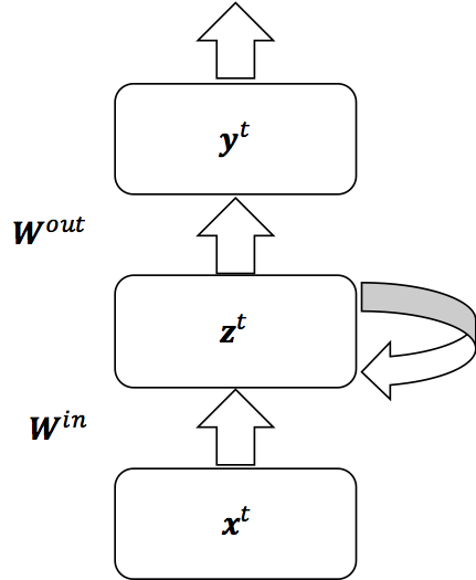
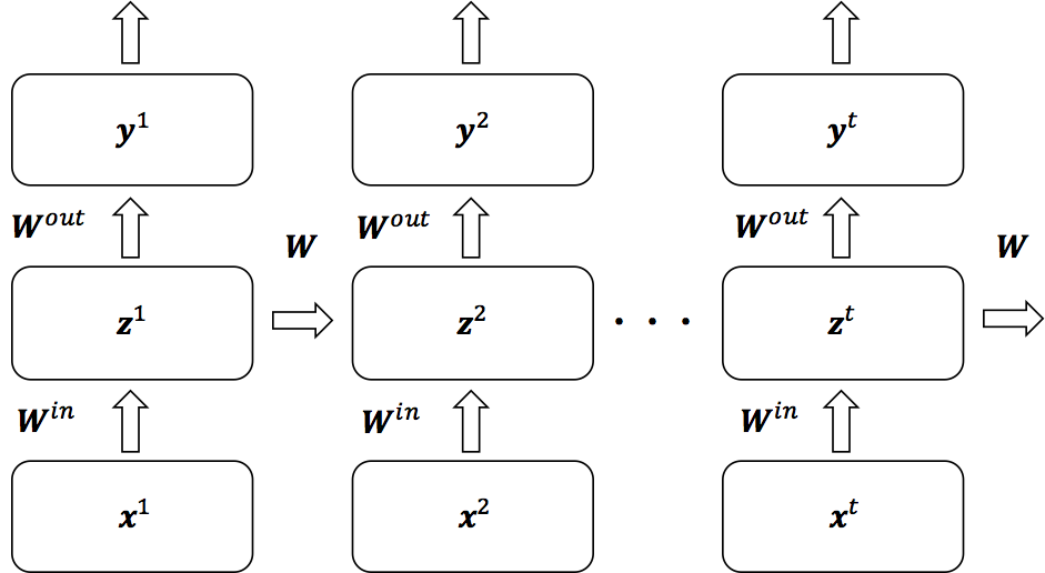
以上の図を時間で展開したものは次のようになる。1つ前の時間の重みが次の時間にフィードバックされていることが分かる。
TensorFlowにおいてzの部分はユニットセルとして扱われ、LSTMやGRUと呼ばれる構造をセルとして指定することができる。
サンプルコード
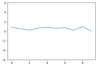
次のようなパターンを波形をクラス分類するニューラルネットを作成する。
クラス1の例
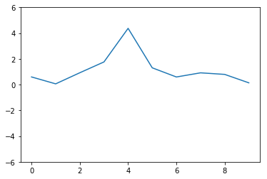
クラス2の例
クラス3の例

TensorFlowにおいて利用できるRNNのセルは次のようになっている。
BasicRNNCellBasicLSTMCellLSTMCellGRUCell
今回はBasicRNNCellを使用する。また、誤差関数には中間層の最終時間における出力(以下のコードでいうoutputs[-1])を用いて出力層の定義を行う。
#!/usr/bin/env python
# coding: utf-8
from __future__ import absolute_import
from __future__ import division
from __future__ import print_function

import random
import numpy as np
import tensorflow as tf
from tensorflow.contrib import rnn

random.seed(777)
np.random.seed(777)
tf.set_random_seed(777)

# パラメーター
N_CLASSES = 3  # クラス数
N_INPUTS = 1  # 1ステップに入力されるデータ数
N_STEPS = 200  # 学習ステップ数
LEN_SEQ = 10  # 系列長
N_NODES = 64  # ノード数
N_DATA = 1000  # 各クラスの学習用データ数
N_TEST = 1000  # テスト用データ数
BATCH_SIZE = 20  # バッチサイズ

# データの準備
def gen_non_pulse(len_seq):
    """波を持たない系列データを生成する"""
    ret = np.random.rand(len_seq)
    ret = np.append(ret, 0)
    return ret.reshape(-1,1)

def gen_pulse(len_seq, positive=True):
    """波を持つ系列データを生成する"""
    seq = np.zeros(len_seq)
    i = random.randint(0, len_seq-3)  # 波を立てる位置
    w = random.randint(1, 4)
    w = w if positive else w * (-1.)
    e = 3 if positive else -3
    l = 1 if positive else 2  # ラベル
    seq[i], seq[i+1], seq[i+2] = w, w+e, w
    noise = np.random.rand(len_seq)
    ret = seq + noise
    ret = np.append(ret, l)  # ラベルを加える
    return ret.reshape(-1,1)

def gen_dataset(len_seq, n_data):
    class_01_data = [gen_non_pulse(len_seq) for _ in range(n_data)]
    class_02_data = [gen_pulse(len_seq, positive=True) for _ in range(n_data)]
    class_03_data = [gen_pulse(len_seq, positive=False) for _ in range(n_data)]
    dataset = np.r_[class_01_data, class_02_data, class_03_data]
    np.random.shuffle(dataset)
    x_ = dataset[:,:10]
    t_ = dataset[:,10].reshape(-1)
    return x_, t_

x_train, t_train = gen_dataset(LEN_SEQ, N_DATA)  # 学習用データセット
x_test, t_test = gen_dataset(LEN_SEQ, N_DATA)  # テスト用データセット

# モデルの構築
x = tf.placeholder(tf.float32, [None, LEN_SEQ, N_INPUTS])  # 入力データ
t = tf.placeholder(tf.int32, [None])  # 教師データ
t_on_hot = tf.one_hot(t, depth=N_CLASSES, dtype=tf.float32)  # 1-of-Kベクトル
cell = rnn.BasicRNNCell(num_units=N_NODES, activation=tf.nn.tanh)  # 中間層のセル
# RNNに入力およびセル設定する
outputs, states = tf.nn.dynamic_rnn(cell=cell, inputs=x, dtype=tf.float32, time_major=False)
# [ミニバッチサイズ,系列長,出力数]→[系列長,ミニバッチサイズ,出力数]
outputs = tf.transpose(outputs, perm=[1, 0, 2])

w = tf.Variable(tf.random_normal([N_NODES, N_CLASSES], stddev=0.01))
b = tf.Variable(tf.zeros([N_CLASSES]))
logits = tf.matmul(outputs[-1], w) + b  # 出力層
pred = tf.nn.softmax(logits)  # ソフトマックス

cross_entropy = tf.nn.softmax_cross_entropy_with_logits(labels=t_on_hot, logits=logits)
loss = tf.reduce_mean(cross_entropy)  # 誤差関数
train_step = tf.train.AdamOptimizer().minimize(loss)  # 学習アルゴリズム

correct_prediction = tf.equal(tf.argmax(pred,1), tf.argmax(t_on_hot,1))
accuracy = tf.reduce_mean(tf.cast(correct_prediction, tf.float32))  # 精度

# 学習の実行
sess = tf.Session()
sess.run(tf.global_variables_initializer())
i = 0
for _ in range(N_STEPS):
    cycle = int(N_DATA*3 / BATCH_SIZE)
    begin = int(BATCH_SIZE * (i % cycle))
    end = begin + BATCH_SIZE
    x_batch, t_batch = x_train[begin:end], t_train[begin:end]
    sess.run(train_step, feed_dict={x:x_batch, t:t_batch})
    i += 1
    if i % 10 == 0:
        loss_, acc_ = sess.run([loss, accuracy], feed_dict={x:x_batch,t:t_batch})
        loss_test_, acc_test_ = sess.run([loss, accuracy], feed_dict={x:x_test,t:t_test})
        print("[TRAIN] loss : %f, accuracy : %f" %(loss_, acc_))
        print("[TEST loss : %f, accuracy : %f" %(loss_test_, acc_test_))
sess.close()
実行結果
- TensorFlow 1.0.0
- Python 3.6.0
[TRAIN] loss : 0.923734, accuracy : 0.600000
[TEST loss : 0.941685, accuracy : 0.585000
[TRAIN] loss : 0.763349, accuracy : 0.800000
[TEST loss : 0.758919, accuracy : 0.830333
[TRAIN] loss : 0.634125, accuracy : 0.950000
[TEST loss : 0.596680, accuracy : 0.820333
[TRAIN] loss : 0.443795, accuracy : 1.000000
[TEST loss : 0.487444, accuracy : 0.961000
[TRAIN] loss : 0.488549, accuracy : 0.900000
[TEST loss : 0.406113, accuracy : 0.961667
[TRAIN] loss : 0.286011, accuracy : 1.000000
[TEST loss : 0.295983, accuracy : 0.981000
[TRAIN] loss : 0.249263, accuracy : 1.000000
[TEST loss : 0.236212, accuracy : 0.977000
[TRAIN] loss : 0.182674, accuracy : 0.950000
[TEST loss : 0.185231, accuracy : 0.977000
[TRAIN] loss : 0.163595, accuracy : 1.000000
[TEST loss : 0.173578, accuracy : 0.963667
[TRAIN] loss : 0.196658, accuracy : 0.950000
[TEST loss : 0.145268, accuracy : 0.983000
[TRAIN] loss : 0.086850, accuracy : 1.000000
[TEST loss : 0.120967, accuracy : 0.990000
[TRAIN] loss : 0.108360, accuracy : 1.000000
[TEST loss : 0.098970, accuracy : 0.987667
[TRAIN] loss : 0.090482, accuracy : 1.000000
[TEST loss : 0.081187, accuracy : 0.991667
[TRAIN] loss : 0.072524, accuracy : 1.000000
[TEST loss : 0.075302, accuracy : 0.994667
[TRAIN] loss : 0.073820, accuracy : 1.000000
[TEST loss : 0.065370, accuracy : 0.996000
[TRAIN] loss : 0.062461, accuracy : 1.000000
[TEST loss : 0.055922, accuracy : 0.997000
[TRAIN] loss : 0.055428, accuracy : 1.000000
[TEST loss : 0.050875, accuracy : 0.998333
[TRAIN] loss : 0.033651, accuracy : 1.000000
[TEST loss : 0.042620, accuracy : 0.998333
[TRAIN] loss : 0.024268, accuracy : 1.000000
[TEST loss : 0.040751, accuracy : 0.994667
[TRAIN] loss : 0.077236, accuracy : 1.000000
[TEST loss : 0.048991, accuracy : 0.992000
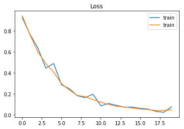
誤差の推移
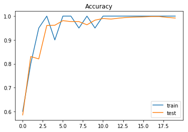
精度の推移
参考
- 岡谷貴之,"深層学習",講談社,2015
- RNNの図は上の本を参考に作成した
- https://www.tensorflow.org/api_guides/python/contrib.rnn
- https://www.tensorflow.org/api_docs/python/tf/nn/dynamic_rnn